Build a Twilight Photometer to Detect Stratospheric Particles

Have you wondered why some sunsets are so spectacular and others so drab? This ultra-sensitive photometer project will allow you to tease out the secrets of twilight and even do serious science by finding the altitude of the dust, smoke, and air pollution that influence the colors of twilight.

With this project you can detect the tiny particles and droplets known as aerosols from 3km (around 10,000 feet) high to well above the top of the stratosphere at 50km (165,000 feet). While the photometer will not detect aerosols below 3km, many of those particles eventually float high enough to be detected. For example, from my Texas site I’ve measured the altitude of smoke from distant fires, haze caused by faraway power plants, and African dust that arrives every summer.

You can even measure the altitude of the sulfuric acid mist that forms an immense blanket 15km–30km high around our entire planet. This stratospheric aerosol layer, which major volcano eruptions can significantly enhance for several years or more, controls the duration of twilights and even influences climate.

Build a Simple Twilight Photometer

The twilight photometer shown in Figure 1 requires no optics and is considerably simpler, smaller, and cheaper than those used by professional scientists. Yet, as shown in Figure 2, it nicely estimates the altitude of dust and smoke clouds from 3km–15km in the troposphere and the permanent aerosol layer at around 15km–30 km in the stratosphere. Instead of a conventional photodiode, the twilight glow is detected by an ordinary 660nm red LED or an 880nm near-infrared LED like those used in remote controls for TVs and appliances.

How It Works

The twilight glow straight overhead is very dim, and the photocurrent it generates in an LED is very small. Therefore it’s important to use an LED installed in clear epoxy. For best results, use an LED that projects a narrow beam when used as a light source. (For details about using LEDs to detect light, see this column.)

The photometer circuit is shown in Figure 3. In operation, the tiny LED photocurrent is amplified billions of times and transformed to a voltage by IC1, a TLC271BIP operational amplifier with a very high-resistance feedback resistor consisting of R1 and R2 in series. Capacitor C1 suppresses oscillation.

The combined resistance of R1 and R2 controls the voltage gain of the amplifier. I have obtained best results using 40-gigohm resistors for both R1 and R2. When only 40 gigohms is required to provide a usable output signal during the 30–45 minute twilight period, switch S2 is closed to bypass R2. High-value resistors can be expensive and difficult to find, but I’ve had good results with Ohmite resistors from Mouser Electronics and Digi-Key. For example, Mouser offers Ohmite’s 40-gigohm axial-lead resistor (MOX-400224008K) for a reasonable $4.27 each. If 40-gigohm resistors aren’t available, use 30- or 50-gigohms.

Planning the Photometer

The twilight photometer should be installed in a metal housing to block electrical noise from power lines and radio signals. I learned this lesson the hard way while testing my first twilight photometers at Hawaii’s Mauna Loa Observatory. The LED can be installed inside the enclosure with a small hole to admit the twilight glow, or inside an open-ended phone or audio plug fitted with a collimator tube and inserted into a jack atop the enclosure. I’ve used both methods and much prefer the external method described here for initial experiments. This allows you to try various LEDs and collimator lengths. After you find the optimum combination, you can install the system inside an enclosure.

Two 9-volt batteries connected in series power the photometer. Because IC1 must not be powered by more than 16 volts, the 18 volts from the two batteries is reduced to 16 volts by Zener diode D1. This arrangement provides the maximum possible output voltage range for a data logging multimeter. If you plan to use a DIY or commercial data logger instead, the circuit’s output voltage must not exceed the data logger’s allowable input voltage. This is typically 5 volts, which means you can power the photometer with a 6-volt battery instead of D1, R3, and the two 9-volt batteries. Both power options are shown in Figure 3. If the logger’s input must never exceed 5 volts, insert a 1N914 diode between the positive battery terminal and IC1.

Assemble the Circuit

The circuit is built on a 1½”×1¼” perforated board with copper traces on the bottom. The prototype board is shown in the open view of the photometer in Figure 4.

For best results, the op-amp’s input (pin 2) should be isolated from the circuit board to prevent dust, fingerprints, and even the board itself from altering the gain of the op-amp. Isolating pin 2 in free air eliminates this problem. The easiest way to do this is to provide an 8-pin IC socket for IC1. Before inserting IC1 into the socket, bend pin 2 straight out so that it doesn’t touch the socket when the other seven pins are inserted.

The next two steps are tricky, so refer to Figure 5 and take your time. First, solder the input side of R1 and C1 directly to pin 2. Then solder a wire directly between pin 2 and the LED cathode (–) terminal of the phone or audio jack.

Install the Circuit in an Enclosure

After the circuit board is assembled, clean the surfaces of R1, R2, and IC1 with a cotton swab dipped in alcohol. Then install the circuit board atop a pair of insulated standoffs inside a metal enclosure as shown in Figure 4. The photometer described here was installed in a Bud Industries CU-124 enclosure. A larger enclosure can be used, as can various metal containers sold by craft stores. If you use two 9-volt batteries (as shown in Figure 4), secure them in place with an angle bracket.

Figure 6 shows a pair of LED-collimator assemblies made from a gas coupler fitting and an aluminum or brass tube. The LED is inserted into an LED socket (optional) soldered to 1/8″ phone plug terminals or soldered directly to the phone plug. (IMPORTANT: Be sure to observe polarity.) The phone plug is pushed into the open end of the lower coupler fitting and secured in place with a rubber O-ring.

You can omit the gas coupler if the plug’s cap will slip over the LED, which means its leads must be clipped close and carefully soldered. Insert the open end of the plug into an appropriate collimator tube. A collimator length of 3″–4″ should provide a field of view of around 5 degrees. As shown in Figure 6, the length of the collimator can be increased or decreased with a short length of heat-shrink tubing.

Using the Photometer

On a clear day 10 minutes before sunset or 45 minutes before sunrise, place the photometer facing straight up on a level surface outdoors well away from light sources. A bubble level mounted atop the photometer will simplify alignment. If necessary, use shims to level the photometer. For best results, connect the photometer output to a data logging multimeter or a standalone DIY or commercial logger (Onset 16-bit HOBO UX120 or similar) and record data at 1-second intervals. If you don’t have a logger, read the output voltage manually from a multimeter at 10- or 15-second intervals and enter the exact time and output voltage into a notebook or audio recorder. Automatic logging is preferable, but the manual method has been used for half a century.

The raw twilight signal should provide a smooth curve when plotted on a graph of time vs. signal. Far more significant is a graph that plots the rate of change in the data against the elevation of the twilight glow. Part 2 of this project below will explain how to process your data so that it accounts for these parameters and reveals the altitude of aerosols over your location. Learn much more about the science of twilight photometry.

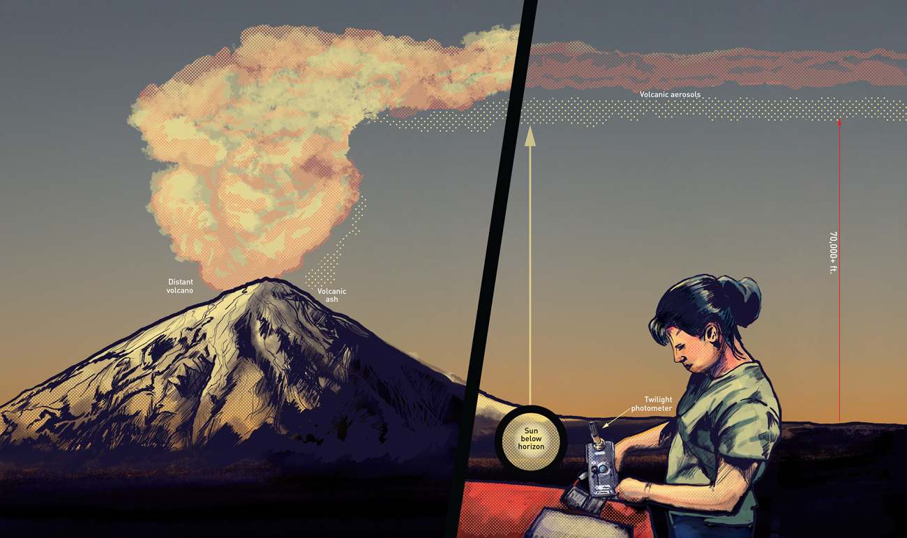
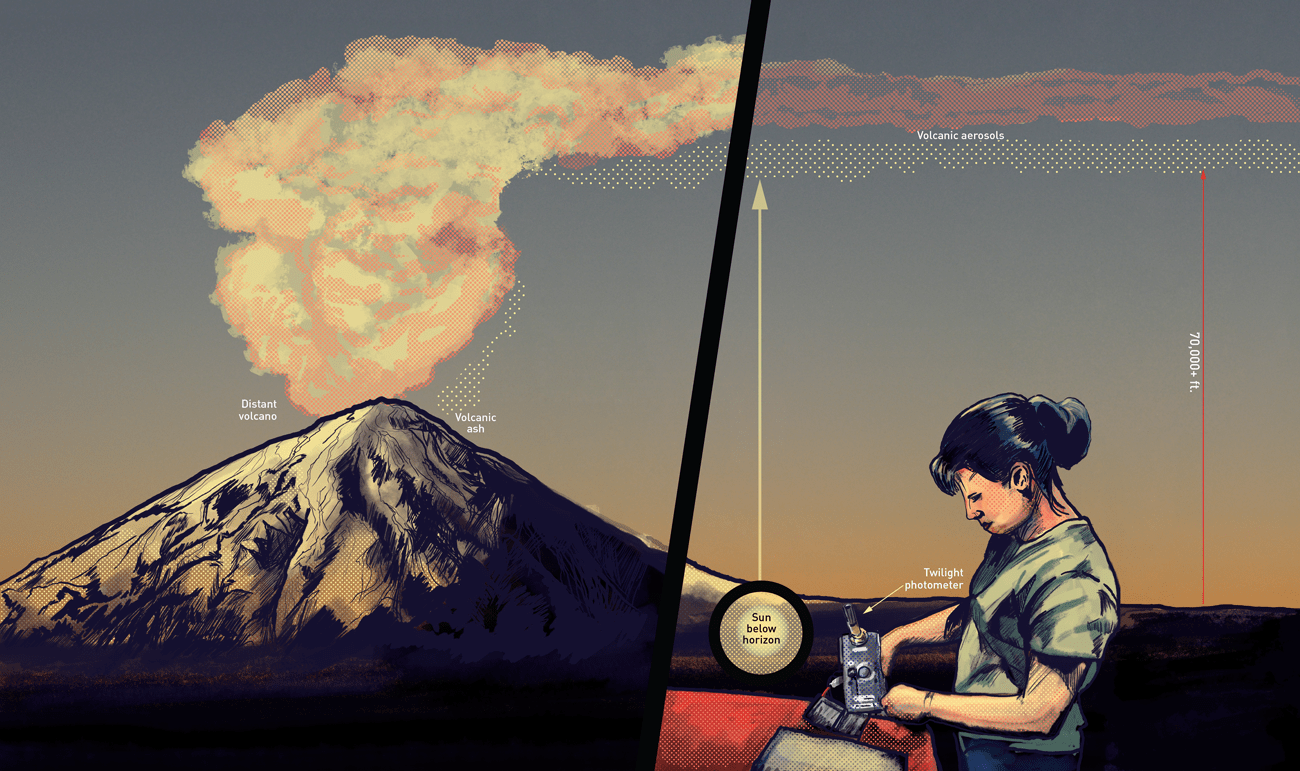
Measure the Altitude of Dust, Smog, Smoke, and Volcanic Aerosols

Next time a Pinatubo-class volcano erupts, amateur scientists will be able to track the height of its aerosol cloud. So far I’ve shown how to make an ultra-sensitive DIY twilight photometer. Now I’ll show how to use a computer spreadsheet to manage and graph your photometer data so you can find the approximate altitude of layers of smoke, dust, smog, and volcanic aerosols in the atmosphere.

The Twilight Glow

If you’re looking toward the sun when it’s just below the horizon, you are at the edge of Earth’s shadow (Figure 7). You can see Earth’s shadow for 10 or so minutes after sunset or before sunrise by looking opposite the sun. If the sky is clear, a pink band will form a wide arc over the horizon. This is the antitwilight glow. The gray or purplish sky below the arc is in the shadow of the Earth.

After sunset the antitwilight arc rises higher in the sky; the opposite occurs during sunrise. Because the atmosphere becomes less dense with altitude, the sky you see when looking straight up during this time is brightest just above Earth’s shadow. Therefore, the intensity measured with a twilight photometer is highest just above the top of Earth’s shadow.

This means that the twilight intensity at any given time is approximately correlated with the height of Earth’s shadow. If sufficiently dense aerosol layers are suspended in this region, the change they cause in the twilight signal can be detected and plotted (Figure 8).

Preparing the Twilight Photometer

It’s important to adjust your twilight photometer to measure the widest possible range of twilight intensities. Ideally we’d do this by rotating a potentiometer shaft, but that’s not feasible with our twilight photometer, because inserting a pot between the LED light sensor and the input to the op-amp might introduce noise. (And I’m unaware of inexpensive pots having a resistance of tens of gigohms.)

The photometer includes two gain resistors, R1 and R2, connected in series, and switch S2 connected across R2. Closing S2 cuts the gain in half. This provides an X1 and X2 gain control. You can alter the gain even more by using different resistances, but this can become expensive.

A simple way to fine-tune the sensitivity of a twilight photometer is to alter the length of the collimator tube installed over the LED. Start with a 5″–6″ length of heat-shrink tubing for the collimator tube, then increase the photometer’s sensitivity by clipping off short segments of the tube to allow more light to enter it, until the photometer output is slightly below the maximum voltage allowed by your data logger. This should be done a few minutes before sunset. You’ll need at least one twilight session to find the optimum length of the collimator tube. You can then replace the heat-shrink with a permanent piece of tubing.

Data Logger Selection

You can manually record your data at 15- to 30-second intervals, but automatic logging at 1-second intervals is much better. For this you’ll need to connect the output of the twilight photometer to a 16-bit or higher resolution data logger. I’ve had good results with Onset’s HOBO UX120, a 16-bit, 4-channel analog logger. I’ve also used the Unisource DM620, a 50,000-count data logging digital multimeter. Many other data loggers and 50,000-count logger DMMs are also available. Just be sure the software is compatible with your computer.

The Twilight Photometer Spreadsheet

I’ve built a custom spreadsheet that manages and graphs your twilight data while saving you from having to solve many equations (Figure 9). You can download it for free, and follow the detailed instructions for using it. The spreadsheet was developed in Microsoft Excel and converted to free LibreOffice. It has 6 pages:

1. Analysis. This sheet calculates the times of sunset and sunrise, sun position, and height of Earth’s shadow. It also calculates the derivative of the data (its change over time), averages it (to smooth it), and creates the charts displayed on Sheet 2. References are provided to acknowledge those who devised twilight photometry.
2. Charts. This sheet shows graphs of the altitude of Earth’s shadow versus the raw data (linear and logarithmic) and the derivative (intensity gradient) of the data.
3. Satellite. Satellite and aerosol forecast images are pasted here. Satellite images show any clouds that might be present. The aerosol models predict the distribution of dust, smoke, and smog.
4. Soundings. This is an optional sheet for upper air soundings from weather balloons launched closest to your site.
5. Data. The raw data goes here.
6. Readme. Detailed photometer and data analysis instructions are here. Carefully read this sheet before your first twilight session.

The single channel twilight photometer spreadsheet is a subset of a 7-channel version I have used to analyze numerous twilights since 2013. It was developed in Microsoft Excel and converted for use with free LibreOffice. It still runs in Excel and also in Apache OpenOffice, but the graphs on Sheet 2 will need minor fixes, and some of the images on page 3 might not appear.

Please acknowledge the spreadsheet and the Make: twilight photometer developer (that’s me) and Make: magazine in your publications or science projects. And don’t forget to acknowledge the twilight scientists who are cited below and in the spreadsheet.

The spreadsheet is provided “as is.” While I hope it works well for you, it might not, so use it at your own risk. Please send corrections, modifications and improvements, together with your permission to post them online, to me at fmims@aol.com. While the volume of emails I receive may make it difficult to respond to every message, I will definitely read all of them.

Finally, before sending questions, be sure to carefully read all of these instructions, the above articles and the references below. My time is very limited, and chances are your questions may already be answered by these sources.

Acknowledgements

This spreadsheet was inspired and made possible by the pioneering work of Australian twilight science pioneer E.K. Bigg, who devised clever methods for estimating the altitude of Earth’s shadow and for extracting aerosol influences on twilight data. Belgian astronomer Jean Meeus developed and published the equations for calculating the position of the sun for a given date, time and location, all of which are essential for calculating the height of Earth’s shadow. Atmospheric scientist Frederick Volz and former Mauna Loa Observatory director Kendrick Coulson developed various kinds of twilight observation methods that led to my work in this field. See relevant references following these instructions.

Start Here

1. IMPORTANT: Carefully read what follows before beginning your first twilight session.
2. This document explains each spreadsheet page and provides instructions for a twilight measurement session. References are provided at the end.
3. Download two copies of the spreadsheet. Save one with the URL name or whatever title you like. This will be a permanent reference. Save the second one with a dated file name, e.g. “TWILIGHT_06152015_PM [or AM]”. Add your initials or site name if you plan to share data with others. Use the dated spreadsheet for your first and subsequent twilight sessions, each saved with the proper date in the file name.
4. As you enter data and otherwise work with the spreadsheet, periodically save the file. Don’t forget to save it again after you complete the spreadsheet. After saving a completed spreadsheet, I immediately back it up to an external drive for safekeeping.
5. The spreadsheet comes complete with data from an actual twilight session.

Explanations for Each Spreadsheet Sheet

SHEET 1: Analysis

This sheet includes various titles and the two key references responsible for the equations that process the data. This sheet is where you enter your geographic location and the date of the twilight session. Columns A and B are where you paste your data from Sheet 5 (see Sheet 5 for details). The spreadsheet then automatically calculates the times of sunset and sunrise, sun position and azimuth (angle to the sun), and height of Earth’s shadow. It also calculates the derivative of the data (its change over time), averages it (to smooth it) and makes the charts displayed on Sheet 2. The top center of the sheet includes these sections:

SITE: Enter your site location and name here.

UNIT 1: This is an overall description of the twilight photometer (Zenith photometer in Al enclosure with one phone jack for 880nm LED (816nm response) in 80mm brass collimator and 2X and 4X gain switch (20GΩ or 40GΩ) used with a DM620 logger.

SKY: Enter the local sky condition and whether or not the satellite images (Sheet 3) show any clouds along the sun’s azimuth for around 45 minutes after sunset.

1. Enter in the yellow box at top left side of the sheet the date, latitude, longitude, and UTC time distance in hours (-5 = EST, -6 = CST, etc.). Use the formats shown in the spreadsheet for all these data.
2. Check satellite imagery for clouds along the solar azimuth path.
3. Load raw data into columns A (times) and B (voltages) of Sheet 5. Highlight and copy all the times and data at and below the sunset time (see cell D12) and paste it in columns A and B at line 16 on sheet 1.
4. After the times and data have been pasted into Sheet 1, look at the height of Earth’s shadow in cell C16. Is it reasonably close to your geographic elevation? If not:
   1. If the height in C16 is significantly lower than your actual elevation, look down column C until you find your approximate elevation. Highlight all cells in columns A and B at and below the proper elevation in column C and drag all these cells up to row 16.
   2. If the height in C16 is significantly higher than your actual elevation, return to Sheet 5, highlight and copy a range of times and data 10 or so seconds before the sunset time (sheet 1, cell D12). Paste these times and data over the current times and data, check the elevations in column C and try step (b) above.

REFERENCES: Sheet 1 includes two key references (additional references are provided below). Thanks to the authors for making this spreadsheet possible.

1. Solar Position Calculations: The calculations on Sheet 1 for the position of the sun, sunset, sunrise, and so forth are adapted from a NOAA spreadsheet based on the brilliant work of Jean Meeus in his Astronomical Algorithms (Willmann-Bell Inc., 1991, 1998).
2. Earth Shadow Height: As noted above, E.K. Bigg derived a method for estimating the height of Earth’s shadow. His method has since been adapted by various others, including B. Padma Kumari, et al., in “Exploring Atmospheric Aerosols by Twilight Photometry,” Journal of Atmospheric and Oceanic Technology 25, 2008 (1600-1607). Their Equation 2 (p. 1604) is adopted for use in this spreadsheet.

CITATION FOR THIS PROJECT: Hopefully you will make some interesting twilight observations and publish or post them online. If so, be sure to cite the references above and the articles in which this project was published (Forrest M. Mims III, “Measure the Altitude of Dust, Smog, Smoke, and Volcanic Aerosols,” Make: magazine Volumes 44 & 45 2015).

SHEET 2: Charts

This sheet shows 3 graphs of the altitude of Earth’s shadow (in kilometers) versus the linear raw data, the logarithm (base 10) of the raw data and the intensity gradient (derivative) of the data:

• Linear Raw Data: Unless clouds or very thick aerosol layers are present, this plot will be a very smooth curve that gradually falls to the minimum voltage detected by your data logger.
• Logarithmic Data: This plot can sometimes reveal tiny excursions caused by aerosol layers. If any can be seen, you might want to greatly magnify the section of the plot where they occur to study them.
• Intensity Gradient (Derivative): This plot shows the derivative of the data averaged over 60 seconds. Otherwise unnoticeable aerosol data in the linear and log graphs is made visually obvious.

You can easily modify the size, placement and formatting of any or all 3 of the graphs. You can also add new graphs. If you’re an experienced spreadsheet user, you can superimpose plots for different days on the same graph axis in order to see differences.

SHEET 3: Satellite

Satellite and aerosol forecast images are pasted here. Satellite images show any clouds that might be present. The aerosol models predict the distribution of dust, smoke, and smog. Links to the satellite and forecast models I use are provided. This is also a good place to paste photographs (see below).

SHEET 4: Soundings

This is an optional sheet for upper air soundings from weather balloons launched closest to your site. These data will provide the height of the tropopause, the boundary between the top of the tropopause (usually 10km–15 km) and the very dry stratosphere.

SHEET 5: Evening Twilight Data

Post all your raw data here after downloading your data logger. You will later paste in columns A and B on Sheet 1 all the times and data from before sunset onward (or from 45 minutes or so before sunrise). Placing all the raw data on this sheet first provides a backup in case something goes wrong with the data that you paste into Sheet 1.

(or)

SHEET 5: Morning Twilight Data

The twilight spreadsheet is designed for evening twilights, when the glow intensity declines with time. But what if you make observations during morning twilight, when the intensity of the glow increases with time?

My solution to this is to invert morning twilight data after it is entered into Sheet 5:

1. Highlight all the data in columns A and B.
2. Left-click the menu item Data
3. Left-click Sort
4. In the box that appears, Sort key 1 should specify Column A.
5. Select the Descending button
6. Left-click OK

Your data will be almost instantly inverted.

IMPORTANT: Be sure to save your spreadsheet with an AM instead of PM filename (e.g. TWILIGHT_06012015_AM).

How to Conduct a Twilight Session

1. Open Sheet 1 of the Twilight Photometer Spreadsheet Using LibreOffice. Enter the date and the geographic coordinates for your location (use Google Earth, GPS receiver, or smartphone). Sheet 1 will then provide the times for sunset and sunrise and the azimuth (angle) of the sun.
   IMPORTANT: Save the spreadsheet now with a filename that gives the date and AM for morning and PM for evening (e.g. TWILIGHT_06012015_PM). Resave the spreadsheet under its name periodically during the entry of data and after you have completed entering and processing the data. As noted above, after saving a completed spreadsheet, I immediately back it up to an external drive for safekeeping.
2. Check for Clouds. The sky must be free of clouds along the sun’s azimuth for at least 30–40 minutes past sunset (or before sunrise). You can determine if clouds are present by placing a compass (or compass rose outline) centered over your location on a GOES visible light satellite image with the compass north facing north on the satellite image. Check for clouds along the sun’s azimuth angle (westerly at sunset and easterly at sunrise) for about one time zone. You can use a GOES IR2 image, but visible is best. See the annotated GOES image on Sheet 3 of the twilight spreadsheet. Be sure to check the sun’s azimuth, for it changes with the seasons (see D13 on Sheet 1).
3. Activate the Data Logger. If the data logger is launched with a computer, be sure the computer’s time is set to the nearest second. The same applies to a data logging multimeter with built-in clock. Launch the logger shortly before taking it and the photometer outdoors. The logging multimeter can probably be launched outside.
4. Set Up the Photometer. Around 10 minutes before sunset or 50 minutes before sunrise, connect the data logger or multimeter to the photometer. Place the photometer on a flat surface, switch the power switch on, and switch the logger on if it hasn’t already been launched. Use a bubble level to make sure the photometer’s collimator tube is looking straight up at the zenith. If necessary, shim the photometer with coins or homemade wedges while watching the level.
5. Photograph the Sky. While photos are optional, they can prove important if you detect unusual aerosol layers. These are the 3 photos I usually make:
   1. Sunset or Sunrise: The sky over the sun when the sun is a minute or so below the horizon, especially when there are thin bands or thick layers of haze caused by smoke, dust, or smog.
   2. Zenith Sky: The zenith sky straight overhead at sunset or sunrise.
   3. Twilight Glow: The sky over the sunset or sunrise point when Earth’s shadow is around 15km to 20km overhead. (See the elevations in column C of Sheet 1.) This photograph will show a brighter than usual sky glow when there is an abundance of aerosols in the lower stratosphere. The glow will be exceptionally bright following a major volcano eruption that forms a veil of sulfate particles in the stratosphere.
6. Download Satellite and Forecast Images. A typical twilight session is 45–60 minutes. While waiting for the session to end, you can download online satellite and aerosol forecast images and paste them into Sheet 3, which includes suggested URLs. Note that these images are usually filed by UTC. Therefore, if you make an evening twilight measurement in the U.S., the closest sounding time will be at 00 UTC the following day.
7. Download Upper Air Sounding. This optional step provides the height of the tropopause, the boundary between the top of the troposphere and the stratosphere. The stratospheric aerosol layer usually begins in the vicinity of the tropopause, so knowing the tropopause height provides an indication of the accuracy of your photometer measurements. According to the World Meteorological Organization, in 2002 weather balloons were being launched from 824 stations around the world. At stations in the U.S. and many other countries, weather balloons are launched twice a day. You can find sounding data from weather balloons online at URLs given on Sheet 4 of the twilight spreadsheet. Depending on your time zone, the weather balloon flight closest to your location may occur before or after your twilight session with the data being posted online a few hours after the flight. The data for flights from Texas, for example, is usually available a few hours after an evening twilight session.

Here are some suggestions for modifying or advancing your twilight photometry project:

1. Manual Logging. If you don’t have a logger, read the output voltage manually from a multimeter at 10- or 15-second intervals and enter the exact time and output voltage into a notebook or audio recorder. Modify the twilight spreadsheet to plot manually acquired data.
2. Spreadsheet Complexity. Perhaps you can find ways to simplify the spreadsheet and reduce its size. For example, on Sheet 1 you might want to calculate the times in columns F, G, and I only in row 16. You can also save memory space by removing all the equations from each cell after a session has been fully entered. Here’s how: Highlight all cells from row 16 and below on sheet 1, right-click and select Copy, right-click and select Paste Special, check Numbers and Date & Time and click OK. Do this only if you will not be modifying the data, for no calculations will be available thereafter. This is why you should save a second copy of the spreadsheet to use as a template. If you enter data into the reference, save it with its own date to avoid losing the reference template.
3. Tropospheric Aerosol Identification. The Navy and NASA aerosol forecast models linked on Sheet 3 provide information about aerosols over your area. When your gradient plot shows bumps at 5km and 10km, and the models show the presence of both dust and smoke, can you determine which aerosol is most likely to be at each elevation? Hint: The NASA aerosol forecast model linked on Sheet 3 of the spreadsheet includes a 3D model option in which aerosols are visually depicted over a range of selectable atmospheric pressures. You can find tables online that convert pressure to approximate elevation. Apply this conversion to your intensity gradient chart on Sheet 2 and compare with the NASA forecast to get the best guess for what caused bumps in your chart.
4. Stratospheric Aerosol Layer. A series of photos showing the brightness of twilight glows the same number of minutes after sunset or before sunrise can provide interesting indications of stratospheric aerosols.
5. Earth’s Shadow. It has a diffuse edge, so the altitude estimates are only approximate. Some twilight scientists have included information about the resolution of twilight measurements as the altitude changes. Perhaps you can modify the spreadsheet to account for these changes and to provide an estimate of altitude accuracy.
6. Aerosol Tracking Project. Consider a long-term aerosol tracking project to observe what happens over the course of a year or more. Post your findings, charts, and photos on a website linked to this one.
7. Very High Altitude Aerosol Tracking. The spreadsheet is designed to work from several km to 50km, the top of the stratosphere. My data often reach 130km or even higher. While the data at these very high altitudes looks good when plotted in the linear and log charts, it becomes very noisy in the intensity gradient plot. Perhaps you can modify the averaging of the derivatives to reduce the noise. If so, keep a close watch on bumps in the intensity gradient plots at or near 83km. This is the region where meteors often leave behind dust as they are consumed by their passage through the atmosphere.
8. Your Ideas. Think of additional ways to modify or improved this twilight photometer project. Will a green LED work as well as an IR LED in the photometer? (No. Can you determine why?)

Some Twilight Examples

Figure 10 shows the 3 graphs from 2 separate twilights superimposed, to demonstrate how the spreadsheet teases out the aerosol layers in the gradient graph. Irregular graphs are produced when clouds are present along the sun’s azimuth; (Figure 11) shows 3 sky profile charts contaminated by clouds along the azimuth.

Going Further

Twilight photometry is an ideal way to become better acquainted with the upper atmosphere. It’s a useful tool for science fair projects, serious science, and curious sky watchers, especially if a major volcano eruption occurs. The spreadsheet also provides suggestions on how to expand the project and how to use a NASA aerosol model to identify aerosol layers you detect. When the next Pinatubo or Laki blows its top (or even a Villarica or Ontake or Eyjafjallajökull if you live nearby), you’ll be ready.

References

Australian twilight pioneer E.K. Bigg gives a detailed method for calculating the height of Earth’s shadow for a given date, time and location in “Atmospheric stratification revealed by twilight scattering,” Tellus XVI (1964).

Twilight scientists in India and elsewhere have used Bigg’s method in their research, and I have especially relied on B. Padma Kumari, et al., “Exploring Atmospheric Aerosols by Twilight Photometry,” Journal of Atmospheric and Oceanic Technology 25 (2008), http://journals.ametsoc.org/doi/abs/10.1175/2008JTECHA1090.1.

The position of the sun is necessary for calculating the height of Earth’s shadow, and Jean Meeus has provided the details in “Astronomical Algorithms” (Willmann-Bell Inc., 1991, 1998). NOAA has used Meeus’s method in a convenient sun position spreadsheet.

Frederick Volz and R.M. Goody conducted significant twilight science. They and most other early twilight scientists pointed their photometers at various angles above the horizon (e.g., 20 degrees) since this provided a stronger signal than the zenith sky. Their classic paper is “The Intensity of the Twilight and Upper Atmospheric Dust,” Journal of Atmospheric Science 19, 1962 (385–406).

Kendrick Coulson, a former director of Hawaii’s Mauna Loa Observatory, preferred to point his photometer straight up at the zenith sky. While the signal is greatly reduced at the zenith, the altitude of Earth’s shadow is easier to calculate, and the data are more easily compared with data from other scientists. This is why the zenith method is used in this project. Coulson’s classic book Polarization and Intensity of Light in the Atmosphere (A. Deepak Publishing, 1988) provides invaluable information about detecting aerosols in the atmosphere and twilight photometry. This book is out of print, but you can use Google to find libraries that have it. Coulson’s paper “Characteristics of skylight at the zenith during twilight as indicators of atmospheric turbidity. 2: Intensity and color ratio” was published in Applied Optics 20, Issue 9, pp. 1516-1524 (1981). This paper is behind a paywall, but it’s worth a search in a university library.